Written by: Lorenzo Casalino
Motivation
Distance analysis allows measuring the interatomic distance between two atoms. When this analysis is performed along a Molecular Dynamics (MD) trajectory, it is possible to visualize the time evolution of some relevant distances and take note of their fluctuations. Such information may be precious to gain insights about the stability of the structure or of an important part of the structure, like a catalytic site of an enzyme, where chemical reactions happen, or the active site of a protein, where a drug can bind and exert its action.
Distance analysis can be easily performed with the program cpptraj, which is a
program designed to load and analyze MD trajectories. Cpptraj is a part of the
AmberTools package of the Amber software suite.
Before performing such analysis it is very important to thoroughly
inspect your trajectory in order to select the distances you want to measure.
For this purpose, we will be using VMD (Visual Molecular Dynamics), a molecular
visualization and analysis program designed for biological systems such as
proteins, lipids or nucleic acids.
You are expected to do this tutorial for each replica of all the 6 HSP90 systems you are given.
First part - Trajectory inspection with VMD
Load the trajectories of the three replicas and RMS-fit it to the first frame
-
Enter the folder of the first HSP90 system you are going to inspect. The trajectories are located at
/scratch/bcc2018_trajectories/${BCCID}. You will find the topology file (*.prmtop) and three subfolders, each corresponding to a different replica (md1,md2,md3) containing the respective trajectories. Load and open VMD from a terminal:> module load vmd > vmdWhen VMD starts, two windows will open: the VMD Main window and the OpenGL Display window. Remember which Terminal window is the one where you have launched VMD.
-
The first step is to load the trajectory of the system. To do this, in the VMD Main window, choose
File > New Molecule.... This opens theMolecule File Browser. Use theBrowse...button to find the topology file (*.prmtop) in the current directory and the open it. Check that in theDetermine file typebox “AMBER7 Parm” has been automatically detected. In order to actually load the file, you have to press theLoadbutton. Do not close theMolecule File Browserwindow because we also need to load the trajectory file. Click on theBrowse...button to find the trajectory file (*.nc) of the first replica in the/md1subdirectory and then open it. Check that in theDetermine file typebox “NetCDF (AMBER, MMTK)” has been automatically detected. Press Load to load the entire trajectory. You have just loaded the trajectory of the first replica.Next, close the
Molecule File Browserand load the remaining two replicas.Ultimately, in the
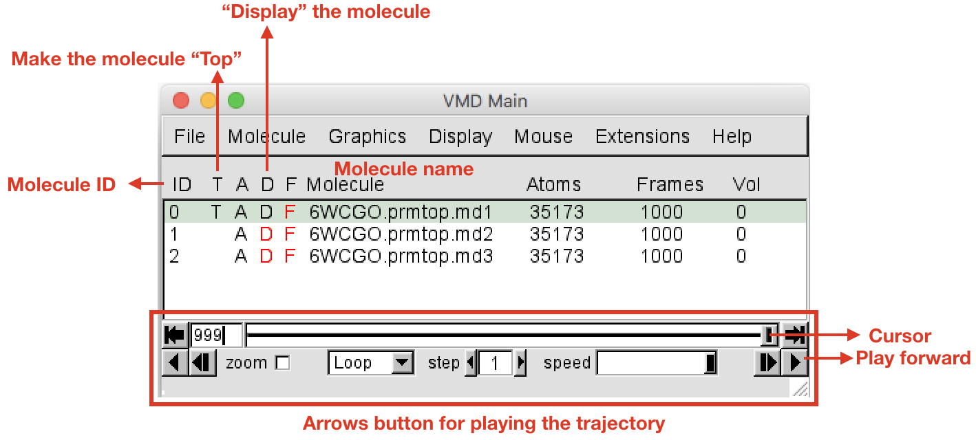
VMD Mainwindow, you should see the three loaded trajectories with three different IDs (0, 1, 2). Click with the left button on the name of the first trajectory to select it, right click to rename by appending.md1to the current name. Do the same for the other replicas adding.md(2/3). In theOpenGL Displaywindow you can see the three molecules (and trajectories) all displayed at the same time. To display only the first one (.md1), in theVMD Mainwindow double click on the “D” letter on the left of.md2and.md3molecules (the letter will become red, meaning that the molecule is not displayed). Now you should see only the first replica md1. Double click under the “T” letter (still in the VMD Main window, on the left of the molecule name) in order to make.md1the “Top” molecule. You must have a situation like the one represented in Figure 1. The trajectory can be played using the arrow buttons at the bottom of theVMD Mainwindow (Figure 1). The speed can be adjusted with the slider in the bottom right hand corner.
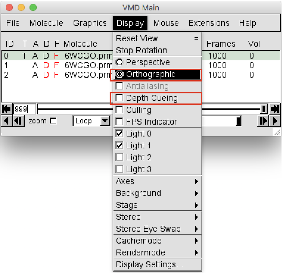
- Before playing around with the trajectory, in the
VMD Mainwindow go toDisplayand change the view from “Perspective” to “Orthographic”. Then deselect “Depth Cueing”, as shown in Figure 2.
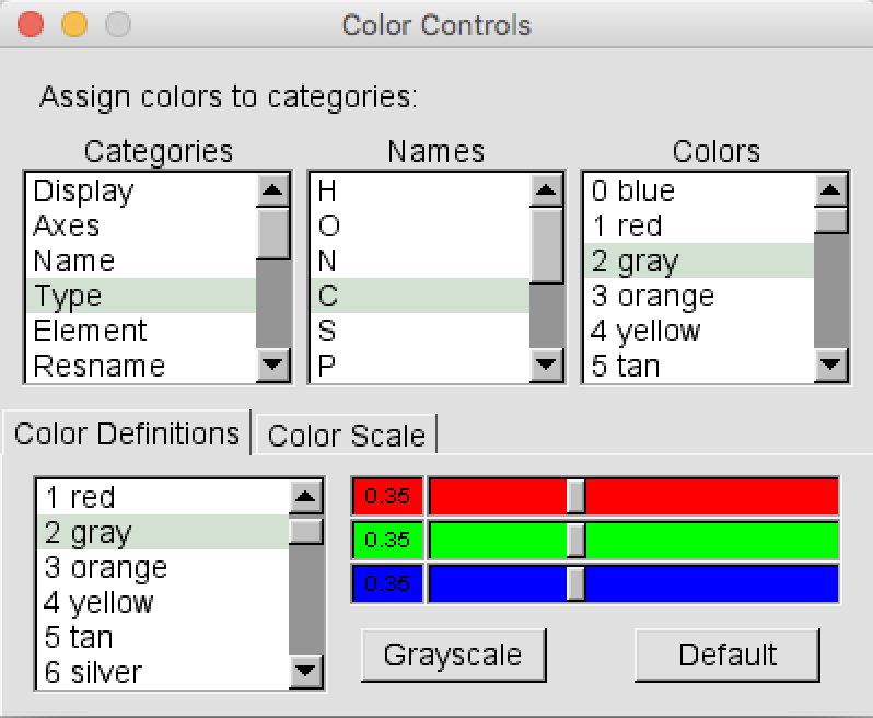
- In the VMD Main choose
Graphics > Colors. A new window calledColor Controlswill open (Figure 3). In the “Categories” left panel select “Type”, then in the central “Name” panel select “C” and finally in the “Colors” right panel select “6 Silver”. Close theColor Controlswindow.
- To properly visualize the trajectory we have to remove the translation and
rotation motions of the system by fitting the trajectory of the heavy atoms
(proteins + ligand) onto the first frame, which is used as a reference. In order
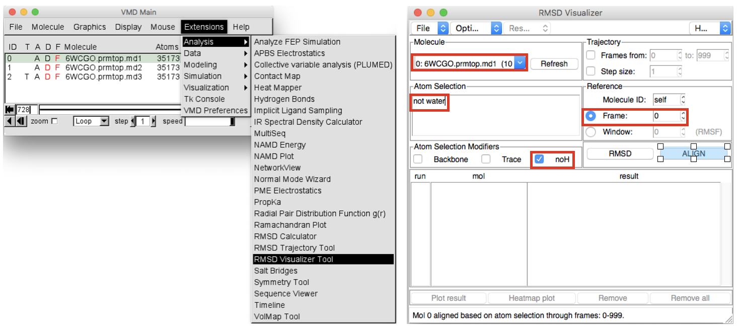
to do so in the VMD Main window go to
Extensions > Analysisand chooseRMSD Visualizer Tool(Figure 4). In the “Molecule” box first select the ID 0 (first replica), then in the “atom selection” box write “not water” and select “noH” in the box below. Select Frame 0 as “Reference” and finally click on the ALIGN button to run the alignment. Do the same also for the ID 1 (.md2) and ID 2 (.md3) molecule, selecting them from the “Molecule” box
Atom selections, visual inspection and features measuring
- Now that you have loaded and aligned all the replicas, you have to choose an
optimal visualization of the protein and the ligand. In order to do so, in the
VMD Main window choose
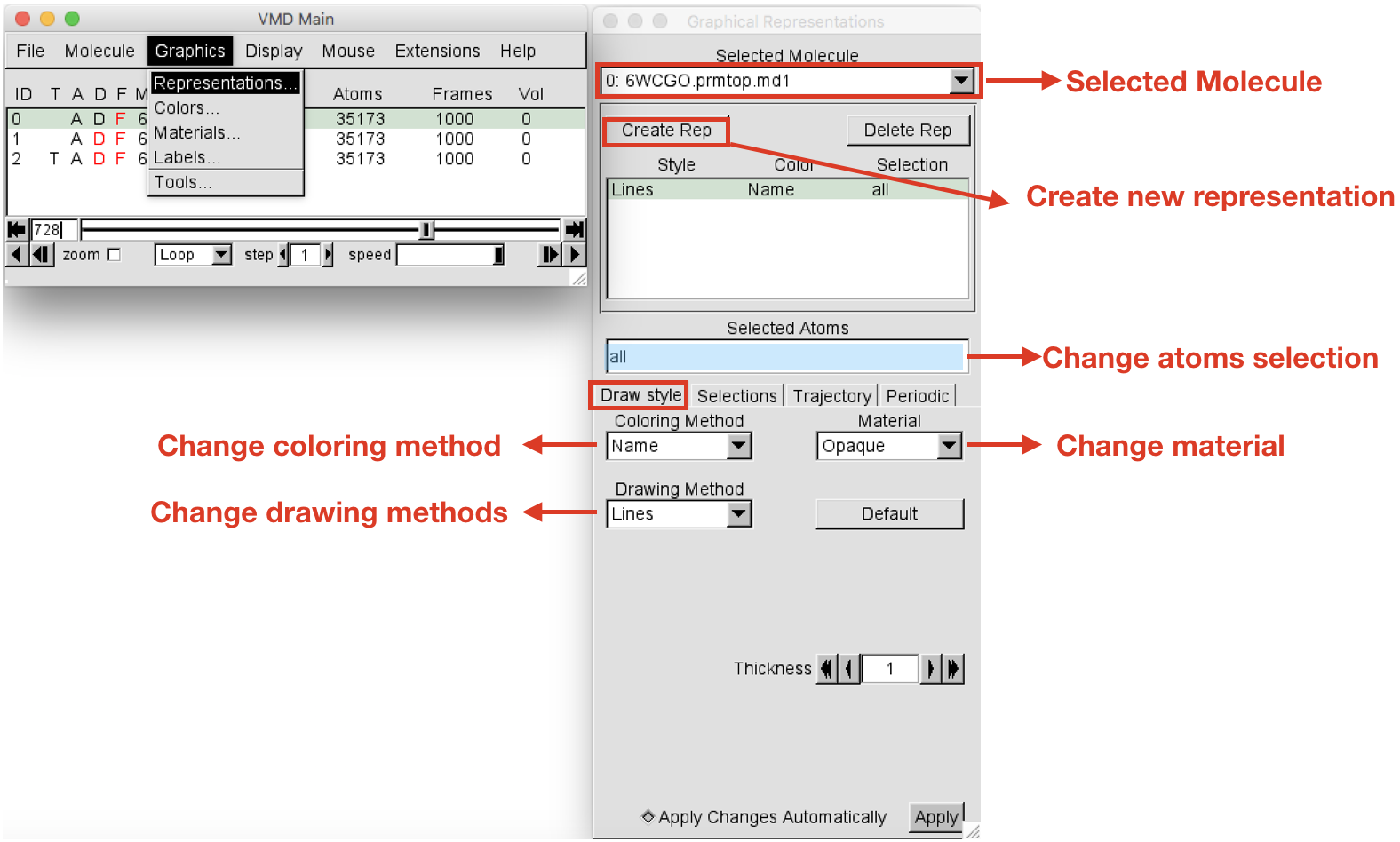
Graphics > Representation. TheGraphical Representationswindow will open (Figure 5). When you open this window, the default atom representation of Molecule 0 (always check for which molecule you are creating representations in the “Selected Molecule” box located at the top) is “all”, meaning that all the atoms of your system are shown as Lines. Select the current representation “all” and change it by typing “protein” (you can do it in the Selected atoms box). Press return. Then change the drawing method to “New Cartoon” to show the secondary structure of the protein. Leave the Coloring Method set to “Name”.
-
Let’s create now the representation for the ligand. Click on the Create Rep button on the top left corner to add a new representation. It will create and identical representation as the last created. Select the newly created representation and change the Selected atoms to “resname LIG”. Note that each system will have a different resname for the ligand, so in place of “LIG” write the actual residue name (“resname”) of the ligand of the system under analysis. Press return. Change the drawing method to “CPK” and the Coloring Method to “Type”. At this point you should have your protein in cyan new cartoon and the ligands represented as C-silver CPK.
-
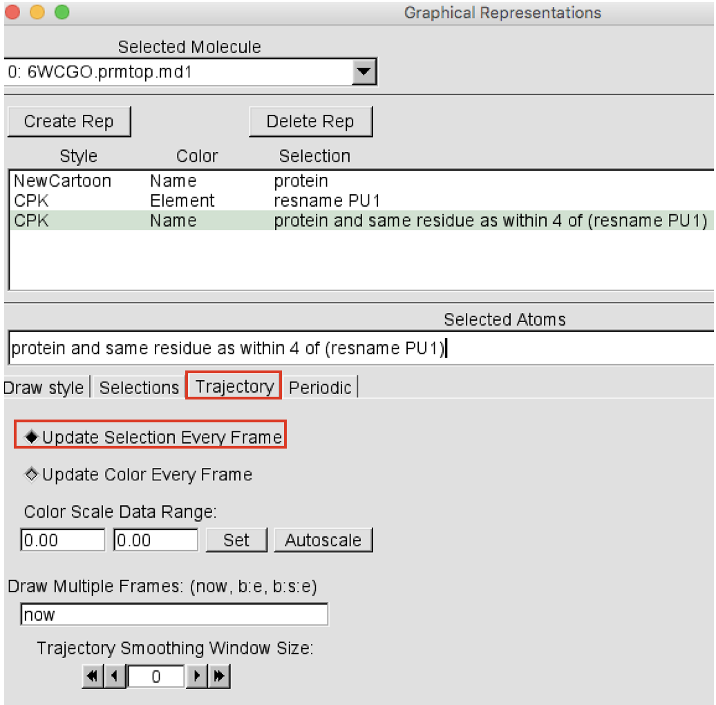
Create now a third representation showing the protein residues that during the trajectory end up being within 4 Å of the ligand(s). This is a distance cutoff that is useful to see the residues that might interact with the ligand. Click on the Create Rep button on the top left corner to add a new representation. Select the newly created representation and change the Selected atoms to “protein and same residue as within 4 of (resname LIG)”. Press return. Change the drawing method to “CPK” and leave the Coloring Method set to “Name”. Now, in order to update this selection at each frame of the trajectory, always in the Graphical Representations window click on the Trajectory button and select “Update Selection Every Frame” (Figure 6).
-
Create a representation for the water molecules that during the trajectory end up being within 2.5 Å of the ligand(s), i.e. at h-bond distance. Click on the Create Rep button on the top left corner to add a new representation. Select the newly created representation and change the Selected atoms to
(resname WAT
and name O H1 H2) and same residue as within 2.5 of (resname LIG)
. Press return. Change the drawing method to “CPK” and leave the Coloring Method set to “Name”. Now, in order to update this selection at each frame of the trajectory, always in theGraphical Representationswindow click on the Trajectory button and select “Update Selection Every Frame”. In theOpenGL Displaywindow, you can now view the ligand depicted as C-silver CPK, the secondary structure of the protein in cyan and the residues within 4 Å of the ligands as C-cyan CPK and all the water molecules at h-bond distance. Play around with the trajectory using the arrow buttons. -
Clone these representations to the other 2 replicas. In order to do this, in the
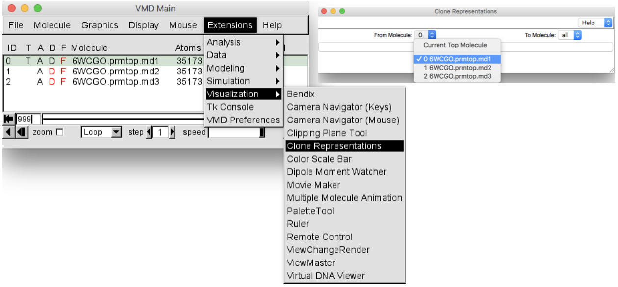
VMD Mainwindow selectGraphics > Representation > Clone Representations. TheClone representationswindow will pop up. Select the.md1molecule (ID 0) from the “From Molecule” box and leave “all” in the “To Molecule” box (Figure 7). In this way all the representations set for the first replica will be set also for the other two replicas.
- Interact with the molecule. Before proceeding with any analysis, it’s always a good
habit to interact with your system. In VMD you can do it in a variety of ways.
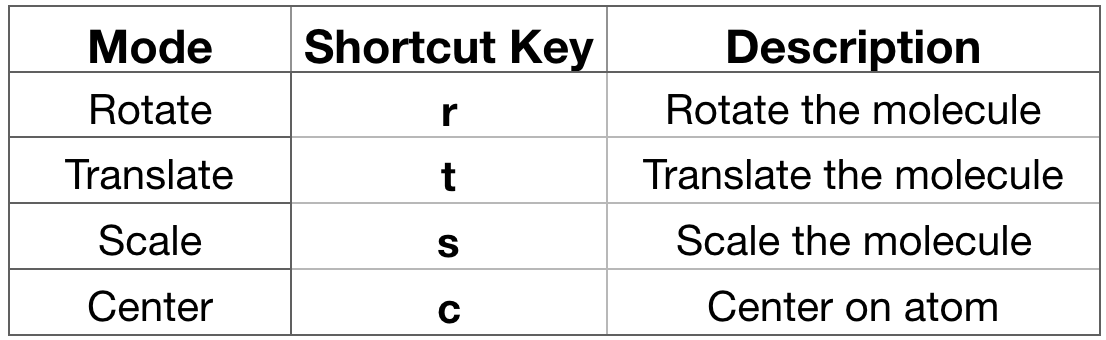
You can rotate, translate and scale (zoom) the molecule. Each of these
interactions modes can be accessed via the Mouse menu in the VMD Main window or
using a shortcut key listed below (Figure 8, strongly suggested). Go on the
OpenGL Displaywindow and drag the mouse with the left click hold. By default, VMD starts in Rotate Mode. You can rotate your molecule. If you press “t” then you enter Translate Mode where you can translate your molecule by dragging the mouse with the left button.
Q1: Try to find an optimal visualization of the active site.
-
Save the visualization state of the system by choosing, in the VMD Main window,
File > Save Visualization state...A new window will open and, in the box beside the word “Filename”, find your own folder where you have permission to write and save it asstate_BCCID.vmd. This will be the name of your state. Press OK button. You can recover this state at a later time from the VMD Main window,File > Load Visualization state.... It’s good practice to save as you go in case VMD crashes while you are working. -
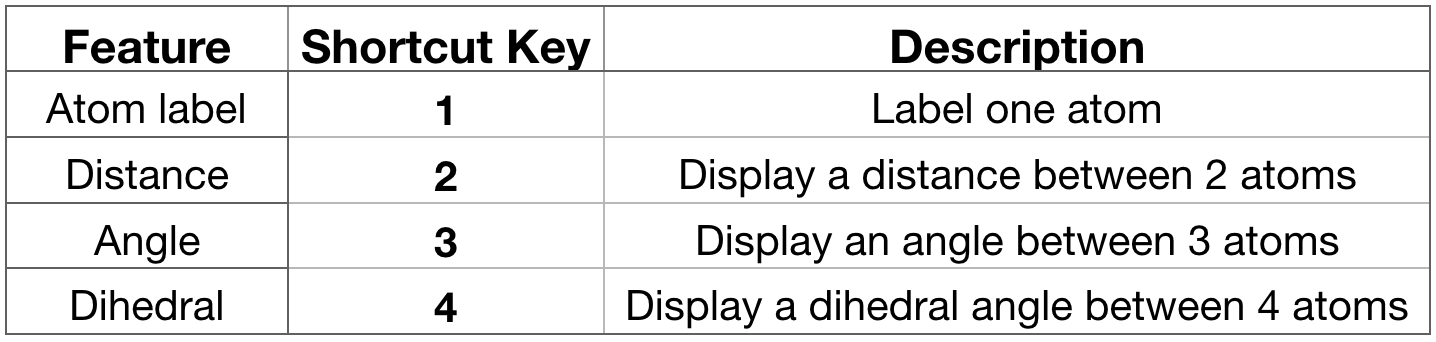
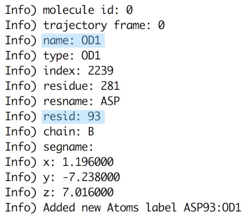
Label atoms, distances, angles. You can place labels on the atoms to display their name and IDs and also to display the distance between two atoms or the angle formed by three atoms and the dihedral angle formed by four atoms. To do so, select the particular feature you would like to label from the
OpenGL Displaywindow using a shortcut key as listed below in Figure 9.If you press “1” and then click over one atom, the atom label will appear. If you press “2” and then consecutively click over 2 atoms, the distance between these 2 atoms will be displayed in white. If you press “3” and then click over 3 atoms, the angle between these 3 atoms will appear in yellow. IMPORTANT: every time you select one atom, in the
Terminalwindow (the one from where you have launched VMD) you will see all the information related to this atom as atom name, type, resname, index, resID, residue, chain, the actual frame and x,y,z coordinates (Figure 9).
Q2: Are there any relevant changes in the overall structure between the first frame and the last frame? Q3: Are there any water molecules interacting with the ligands or bridging the ligand and the protein?
Identification of relevant distances
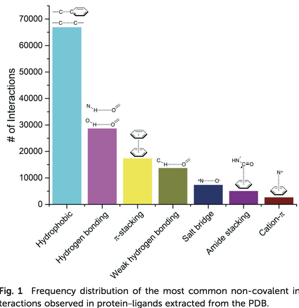
Research on hydrogen bonds and other contacts between the ligand and the protein (or water). A recently published study (R. F. de Freitasa and M. Schapira, Med. Chem. Commun., 2017, 8, 1970-1981) analyzed 11’016 PDB X-ray structures of small-molecules in complex with proteins, with a resolution ≤ 2.5 Å, clustering the most frequent ligand/protein atom pairs in 7 recurrent interaction types. This distribution is shown in Figure 11. Taken together these results show that hydrophobic and electrostatic-based (hydrogen bonds and salt-bridge) interactions are a driving factor for the increased ligand efficiency.
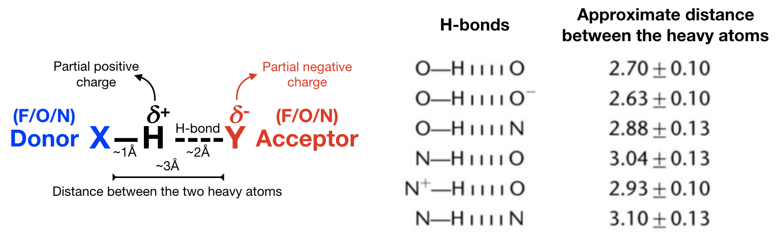
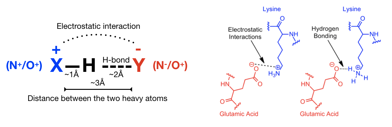
a) Hydrogen bonds (Figure 12) are an important non-covalent structural force (primarily electrostatic in nature) in molecular systems. They are formed when a single hydrogen atom is effectively shared between the heavy atom it is covalently bonded to (the hydrogen bond donor) and another heavy atom (the hydrogen bond acceptor). Both the donor and acceptor atoms are typically quite electronegative. The general rule of thumb for determining whether atoms can form an hydrogen bond is “hydrogen bonds are FON”, i.e. hydrogens bonded to F, O, and N atoms can be donated, and F, O, and N atoms can be acceptors (although there are exceptions). Usually, the angle Acceptor-Donor-Hydrogen is an acute angle comprised between 0 and 20 degrees.
b) Salt bridge (Figure 13): A salt bridge can be defined as an interaction between two groups of opposite charge in which at least one pair of heavy atoms is within hydrogen bonding distance. A salt bridge is a combination of two non-covalent interactions: hydrogen bonding and electrostatic interaction. Salt bridges can contribute to protein stability, molecular recognition and catalysis. Salt bridges usually involve charged amino acids like Asp or Glu (negative) and His, Arg, or Lys (positive) and display extremely well-defined geometric preferences.
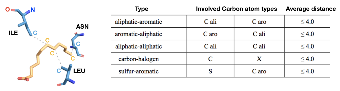
c) Hydrophobic contacts (Figure 14): hydrophobic interactions are the most common interactions in protein–ligand complexes. Hydrophobic interactions comprise contacts between a carbon (aliphatic or aromatic) and a carbon (aliphatic or aromatic), halogen or sulfur atom. The most populated group is the one formed by an aliphatic carbon (from alanine, leucine, isoleucine, valine) in the receptor and an aromatic carbon in the ligand. However, interactions involving an aliphatic or aromatic (for example from a phenylalanine) carbon in the protein and a chlorine/fluorine in the ligand are the second most common hydrophobic contacts, followed by interactions involving a sulfur atom from the side chain of a methionine and an aromatic carbon from the ligand. Also, contacts involving an aromatic or aliphatic carbon in the receptor and an aliphatic carbon in the ligand are common. In general, leucine, followed by valine, isoleucine and alanine side-chains are the most frequently engaged in hydrophobic interactions.
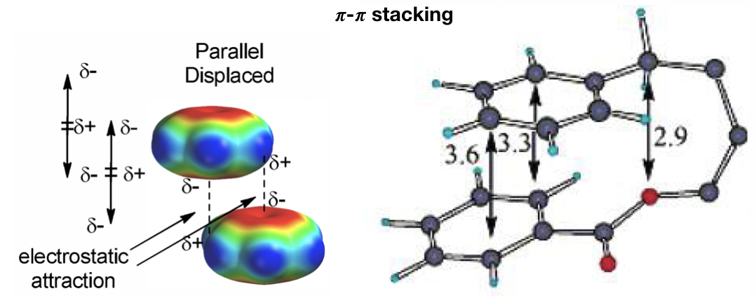
d) 𝝅-𝝅 stacking (Figure 15): 𝝅-interactions can be considered a special case hydrophobic interactions that involves π systems (like aromatic cycle) and they are thought to be a combination of VDW dispersion and electrostatics. They control such diverse phenomena as the vertical base-base interactions which stabilize the double helical structure of DNA, the intercalation of drugs into DNA, the packing of aromatic molecules in crystals, and the tertiary structures of proteins. In particular, 𝝅-𝝅 concerns the direct interactions between two aromatic systems. For example, aromatic amino acids like phenylalanine, tyrosine and tryptophan can do this type of interaction. The T-shaped edge-to-face and the parallel-displaced stacking arrangement predominate.
Q4: Using the distance selection shortcut (“2”), try to dissect how the ligand is interacting (H-bonds, salt bridge, hydrophobic interactions, stacking) with the protein residues (or water molecules). Take advantage of the representations you have drawn before, and possibly draw new ones.
Display window and will help you to better determine which are the possible H-bonds.Take note on your notebook of the distances you consider to be relevant for the
ligand interacting with protein (at least 5), especially h-bonds, reporting the resid, atom
name and the resname of the involved atoms (as in the example below). Report a
few of hydrophobic contacts if you can find them. Pay attention to halogen atoms
of the ligand that might be involved in such interactions. Importantly, in doing
this task consider only the heavy atoms and take note of the distances between
them. For H-bonds and salt bridges consider O and N atoms. For hydrophobic
contacts consider C, S or halogen atoms. For aromatic 𝝅-𝝅 stacking interactions
consider the distance between two C atoms belonging to the two rings. Remember
that you can retrieve the atom information either in the Terminal window (every
time you click on one atom it displays the information) or by looking at the
label that appears above the atom in the OpenGL Display window. Check these
contacts both at the beginning (frame 0) of the trajectory and at the last frame
and check if the ones that are present at the beginning are conserved or not,
and if new contacts form during the simulation.
At the end, on your notebook you should have a list like this:
SYSTEM 1, replica #1 (md1): List of contacts
| # | TYPE | FRAME 0 | LAST FRAME | TYPE | |
|---|---|---|---|---|---|
| 1 | H-bond | 169@OG1 (THR)— 210@N2 (LIG) | V | H-bond | |
| 2 | H-bond | 78@OD2 (ASP) — 210@N5 (LIG) | V | H-bond | |
| 3 | H-bond | 3645@O (WAT) — 210@N1 (LIG) | X | ||
| 4 | 83@C3 (MET) — 210@Cl (LIG) | Hydroph. | |||
| 5 | 147@CZ2 (TRP) — 210@C20 (LIG) | Hydroph. |
Q5: Repeat the same VMD inspection also for the second (md2) and third (md3)
replicas. Remember that you have already uploaded the trajectories, aligned them
to the first frame and cloned the representations from md1. In the Main VMD
window double click on the “D” on the left of the md2 molecule to display it
and un-display molecule (double click on its “D”). Make molecule md2 as the
“Top”. Do the analysis and repeat it afterwards for md3. Report all the
distances as in Q1.
Second part - Distance analysis with cpptraj
Once you have taken note of some relevant distances arising along your Molecular
Dynamics simulations, you are ready to perform the distance analysis. This will
allow you to monitor each single selected distance (among the ones you have
selected) along the trajectory and check its average value and deviation standard.
To perform distance analysis, we will build a bash script that allows performing
this analysis using the cpptraj program. For this aim, the necessary files are
the topology file and the trajectory file of each replica, plus your notes from
the previous visual inspection with VMD.
Create the distance_script.sh to perform the distance analysis, compute average and plot the results
In your personal scratch directory /scratch/${username} create a new folder
called “distance_analysis”, enter into this folder and create six subfolders, one for each of the 6 HSP90 systems (name them with their BCCID). Enter into the folder of the first system you are analyzing and use a text editor,
like gedit, to create the file script_distance.sh:
> mkdir distance_analysis
> cd distance_analysis
> mkdir 6WCGO LLCXM NEQSA OVHRZ TNRT6 VEH1I
> cd 6WCGO/
> gedit script_distance.sh
-
On the first line of the page type:
#!/bin/bash - Define variables for the name of your topology, trajectory, cpptraj input files and output files:
TOP=/scratch/bcc2018_trajectories/6WCGO/6WCGO.prmtop # Topology file (put the whole path) TRAJ1=/scratch/bcc2018_trajectories/6WCGO/md1/6WCGO-Pro01.nc # Trajectory1 (put the whole path) TRAJ2=/scratch/bcc2018_trajectories/6WCGO/md2/6WCGO-Pro01.nc # Trajectory2 (put the whole path TRAJ3=/scratch/bcc2018_trajectories/6WCGO/md3/6WCGO-Pro01.nc # Trajectory3 (put the whole path INPUT1=cpptraj.distance1.in # Cpptraj input file for replica 1 INPUT2=cpptraj.distance2.in # Cpptraj input file for replica 2 INPUT3=cpptraj.distance3.in # Cpptraj input file for replica 3 OUTPUT1=1_distances.dat # Output for replica 1 OUTPUT2=2_distances.dat # Output for replica 2 OUTPUT3=3_distances.dat # Output for replica 3 - Assign a variable the name of each selected distance (use the names reported below as models for yours):
# Define variables for replica 1 distances # DIST1_1=1-hbond-THR169-LIG DIST2_1=1-hbond-ASP78-LIG DIST3_1=1-hbond-WAT3645-LIG DIST4_1=1-hydrophobic-MET83-LIG DIST5_1=1-hydrophobic-TRP147-LIG # Define variables for replica 2 distances # DIST1_2=2-hbond-THR169-LIG DIST2_2=2-hbond-ASP78-LIG DIST3_2=2-hbond-WAT3645-LIG DIST4_2=2-hydrophobic-MET83-LIG DIST5_2=2-hydrophobic-TRP147-LIG # Define variables for replica 3 distances # DIST1_3=3-hbond-THR169-LIG DIST2_3=3-hbond-ASP78-LIG DIST3_3=3-hbond-WAT3645-LIG DIST4_3=3-hydrophobic-MET83-LIG DIST5_3=3-hydrophobic-TRP147-LIG -
Let’s prepare the cpptraj input file for replica 1 (md1). With the command
cat << EOF > $INPUTwe pass a multi-line string (i.e., all the lines up to the line containing the delimiterEOF) to a file called$INPUT1, which is distance_analysis1.in (i.e. for the first replica) i.e. the input file read by cpptraj. The file distance_analysis1.in will contain all the instructions that the program cpptraj needs to perform the analysis:# Cpptraj input file for replica 1 # cat << EOF > $INPUT1 -
From this point, all the lines will end up in the input file distance_analysis1.in, which begins by reading the trajectory file
$TRAJ1from frame 1 to the last:trajin $TRAJ1 1 last # Read the trajectory1 -
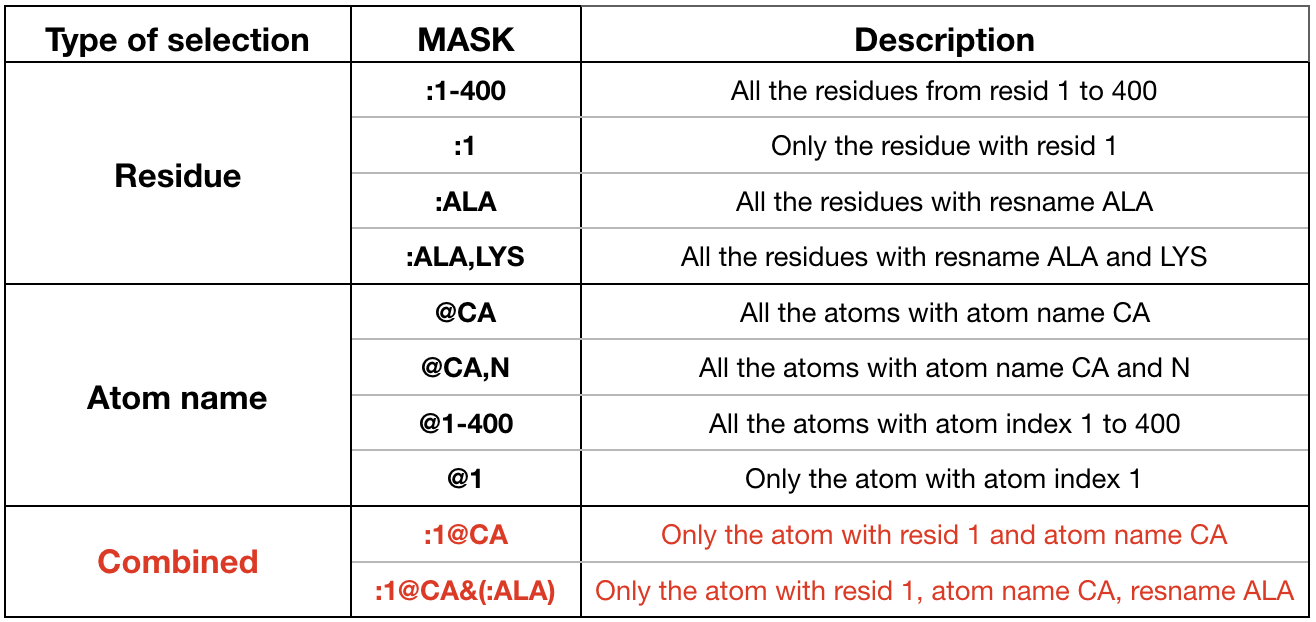
Each frame of the trajectory must be aligned to the first frame (i.e. RMS-fit to first frame), considering only the heavy atoms (no hydrogens) of the solute. In this way we capture only the internal motion, thus removing the global rotation and translation of the system. An atom selection mask must be specified. For example the mask
:1-210&!@H=says that all the residue atoms from 1 to 210 (:1-210) except for the hydrogens (!@H=) are considered:rms first :1-210&!@H= # RMS-fit to frame 1 -
The distance analysis is performed by cpptraj through the command
distance. The commanddistancecalculates the distance between the center of mass of two atoms and it is defined in this way:distance distance_name mask1 mask2 out filename- The distance_name is the name for the dataset of the distance you are interested in. Insert the variable name defined at the beginning (ex.: $DIST1_1).
- The distance is computed between the atom specified in mask1 and the atom defined in mask2. Use the selection mask to specify the 2 atoms. Look at the examples highlighted in red in Figure 15 for the syntax used by cpptraj for defining the two masks of the atoms involved in the distance.
- The output of the analysis is written into a file called filename specified after “out”. Insert the variable name defined at the beginning (ex.: $OUTPUT1 for distances of replica 1). Note that all the distances will be written in the same file, each in a different column.
Insert as many distance commands as many distances you want to analyze. You should have something like:
distance $DIST1_1 :169@OG1 :210@N2 out $OUTPUT1 distance $DIST2_1 :78@OD2 :210@N5 out $OUTPUT1 distance $DIST3_1 :3645@O :210@N1 out $OUTPUT1 distance $DIST4_1 :83@CE :210@Cl out $OUTPUT1 distance $DIST5_1 :147@CZ2 :210@C20 out $OUTPUT1
- Calculate the average (avg command) and standard deviation for each
distance. All the distance datasets are read and their avg and s.d. are
printed to an output file called
1_avg.dat(for replica 1) in column 1 and 2, respectively:avg $DIST1_1 $DIST2_1 $DIST3_1 $DIST4_1 $DIST5_1 out 1_avg.dat - Finish the generation of the input file for replica 1 with EOF marker:
EOF - Now leave a blank line and prepare the cpptraj input file for replica 2 (
$INPUT2). Remember to change all the number “1” to “2”, when it is the case.# Cpptraj input file for replica 2 # cat << EOF > $INPUT2 trajin $TRAJ2 1 last # Read the trajectory2 rms first :1-210&!@H= # RMS-fit to frame 1 distance $DIST1_2 :169@OG1 :210@N2 out $OUTPUT2 distance $DIST2_2 :78@OD2 :210@N5 out $OUTPUT2 distance $DIST3_2 :3645@O :210@N1 out $OUTPUT2 distance $DIST4_2 :83@CE :210@Cl out $OUTPUT2 distance $DIST5_2 :147@CZ2 :210@C20 out $OUTPUT2 avg $DIST1_2 $DIST2_2 $DIST3_2 $DIST4_2 $DIST5_2 out 2_avg.dat EOF - Now leave a blank line and prepare the cpptraj input file for replica 3 (
$INPUT3). Change all the 2 to 3.# Cpptraj input file for replica 3 # cat << EOF > $INPUT3 trajin $TRAJ3 1 last # Read the trajectory3 rms first :1-210&!@H= # RMS-fit to frame 1 distance $DIST1_3 :169@OG1 :210@N2 out $OUTPUT3 distance $DIST2_3 :78@OD2 :210@N5 out $OUTPUT3 distance $DIST3_3 :3645@O :210@N1 out $OUTPUT3 distance $DIST4_3 :83@CE :210@Cl out $OUTPUT3 distance $DIST5_3 :147@CZ2 :210@C20 out $OUTPUT3 avg $DIST1_3 $DIST2_3 $DIST3_3 $DIST4_3 $DIST5_3 out 3_avg.dat EOF - Now leave a blank line and add the following lines to the script to run the
cpptraj program for all the replicas. This will read the topology
$TOPand the input files just generated$INPUT*, printing a log file for each analysis:# Execute cpptraj distance analysis # module load amber/18 # load amber program (and so cpptraj) cpptraj $TOP $INPUT1 > log1 cpptraj $TOP $INPUT2 > log2 cpptraj $TOP $INPUT3 > log3 - Leave a blank line. Finally, we want to plot all the distances of all
the replicas to graphs and produce images (1distances.png, 2_distances.png
and 3 distances.png). To do this we have to add a few more lines to our script.
- To plot the distances we’ll use
Gnuplot. Gnuplot will read an input file that we generate in the same way as we have done for the cpptraj input (through thecat << EOF > gnuplot_1.incommand for replica 1). - In this input we first specify all the graph options (
setcommands). These commands must be copied as they are reported. - Then, always in the input, the
plotcommand will plot the distances (plot '$OUTPUT1'...). In each line you have the name of the distance file ('$OUTPUT1'), followed by the columns you want to plot (u 1:2), meaning the x (column 1 = frame #) and y (column 2 = distance name) axes. Since each distance has been printed to a different column in the$OUTPUT1file, the y column to be read must be changed in order to plot all the distances (1:2, 1:3, 1:4, etc.). After the columns, there are some s pecifics for the line width to be used in the graph (w l lw 3) and the legend name for that distance (title '$DIST1_1'). Each line must terminate with a comma and a backslash (, \), but the last line. Insert as many lines as many distances you want to plot, change the y columns from 2 up to the number of distance you want to plot and remember that the final line should not contain (, \).
# Plot distances replica 1# cat << EOF > gnuplot_1.in set xrange [0:1000] set yrange [0:8] set tics font ", 20" set mxtics set mytics set xtics 0, 100, 1000 set xtics offset 0,-0.2 set ytics 0, 0.5, 8 set border lw 2 set lmargin 11 set rmargin 4 set xlabel offset 0,-1.0 'frame #' font ", 22" set ylabel offset -1.0,0 'distance (Å)' font ", 22" plot '$OUTPUT1' u 1:2 w l lw 3 title '$DIST1_1', \ '$OUTPUT1' u 1:3 w l lw 3 title '$DIST2_1', \ '$OUTPUT1' u 1:4 w l lw 3 title '$DIST3_1', \ '$OUTPUT1' u 1:5 w l lw 3 title '$DIST4_1', \ '$OUTPUT1' u 1:6 w l lw 3 title '$DIST5_1' EOFLeave a blank line and do the same to plot the distances of replica 2 contained in the file ($OUTPUT2):
# Plot distances replica 2# cat << EOF > gnuplot_2.in set xrange [0:1000] set yrange [0:8] set tics font ", 20" set mxtics set mytics set xtics 0, 100, 1000 set xtics offset 0,-0.2 set ytics 0, 0.5, 8 set border lw 2 set lmargin 11 set rmargin 4 set xlabel offset 0,-1.0 'frame #' font ", 22" set ylabel offset -1.0,0 'distance (Å)' font ", 22" plot '$OUTPUT2' u 1:2 w l lw 3 title '$DIST1_2', \ '$OUTPUT2' u 1:3 w l lw 3 title '$DIST2_2', \ '$OUTPUT2' u 1:4 w l lw 3 title '$DIST3_2', \ '$OUTPUT2' u 1:5 w l lw 3 title '$DIST4_2', \ '$OUTPUT2' u 1:6 w l lw 3 title '$DIST5_2' EOFLeave a blank line and do the same to plot the distances of replica 3 contained in the file ($OUTPUT3):
# Plot distances replica 3 # cat << EOF > gnuplot_3.in set xrange [0:1000] set yrange [0:8] set tics font ", 20" set mxtics set mytics set xtics 0, 100, 1000 set xtics offset 0,-0.2 set ytics 0, 0.5, 8 set border lw 2 set lmargin 11 set rmargin 4 set xlabel offset 0,-1.0 'frame #' font ", 22" set ylabel offset -1.0,0 'distance (Å)' font ", 22" plot '$OUTPUT3' u 1:2 w l lw 3 title '$DIST1_3', \ '$OUTPUT3' u 1:3 w l lw 3 title '$DIST2_3', \ '$OUTPUT3' u 1:4 w l lw 3 title '$DIST3_3', \ '$OUTPUT3' u 1:5 w l lw 3 title '$DIST4_3', \ '$OUTPUT3' u 1:6 w l lw 3 title '$DIST5_3' EOFTo launch gnuplot and plot all the distances for the 3 replicas, insert the following lines in your script:
gnuplot -e "set terminal png size 1920,1080 font ',16' " gnuplot_1.in > 1_distances.png gnuplot -e "set terminal png size 1920,1080 font ',16' " gnuplot_2.in > 2_distances.png gnuplot -e "set terminal png size 1920,1080 font ',16' " gnuplot_3.in > 3_distances.pngNote that you can change the font size of the legend by increasing the number from ‘,16’ to ‘,18’ or ‘,20’.
- To plot the distances we’ll use
Launch the script_distance.sh file to perform the distance analysis and check the results
- Good, you have completed your script! Now save your file
script_distance.shby clicking on SAVE button and close gedit. On the terminal, in the distance_analysis/BCCID directory, write the following commands to run the script:> chmod 777 script_distance.sh > ./script_distance.sh -
The script should run smooth and fast (5 seconds). If not, try to understand the error or call someone. You can open the generated png images and inspect the plotted distances with the following command:
> eog -f 1_distances.png 2_distances.png 3_distances.pngBy using the cursor you can move among the 3 images.
Q1: Comment the distance profiles. Are the distance profiles overall stable or do you notice dramatic changes?
Q2: Is there any contact that is stable from the beginning till the end? Where (which frame) do the new contacts form?
Q3: Among the 3 replicas, which are the conserved distances? Take note.
Q4: Open with a text editor the average files (1_avg.dat, 2_avg.dat and 3_avg.dat) and check the averages and standard deviation of the conserved distances selected in Q3. Which distance, among these conserved ones, has the smallest standard deviation (i.e. it’s more stable)? Is the s.d. comparable among the three replicas? Write down the most stable conserved distance and its s.d.
Perform the distance analysis (starting from VMD inspection) for the remaining systems
-
You are done with the first system. Now go into the folder of the system 2 and start from the beginning. Upon visual inspection with VMD, write down the distances, create the distance_analysis folder and copy into this folder the script_distance.sh you have generated for system 1. Don’t forget to modify the script according to the new system, adding or deleting distances, changing their name, tuning the atom selection masks (ligand name…) and so on.
** !!! Before continuing with the next Questions, you need the distance analyses done for all the 6 systems **
Q5: Compare now the 6 HSP90 systems and thus the 6 different ligands. Which of these ligands appear to establish more stable contacts (conserved among the three replicas)? In this analysis consider both the number of conserved contacts, their s.d. and their nature (h-bonds, salt-bridge, hydrophobic, stacking). Indeed, typical energies for salt bridge is ~2 kcal/mol, h-bond ~1 kcal/mol, hydrophobic ~0.7 kcal/mol, stacking 1-3 kcal/mol. Since dG=-2.303RTlogK we can calculate that:
- a single salt bridge interaction might afford a 25-fold increase in affinity
- a hydrogen bond yields a 6-fold increase, similar to 𝝅-𝝅 stacking
- a hydrophobic contact yields a 3.5-fold increase in the binding constant
Q6: Try to correlate all the information gained upon distance analysis with the IC50 values. You were indeed given the IC50 values (in nM) for each ligand. A lower IC50 means higher potency and vice versa. However, as you have done for the RMSD/RMSF analysis, we will express IC50 as pIC50 (pIC50 = -log(IC50)). This means, instead, that a ligand with a higher pIC50 is more potent. To plot the -log(IC50) please first convert the IC50 values from nM scale to M scale (1nm = 0.000 000 001 M = 1E-9 M). After you have done this, in the distance_analysis directory prepare a two-column file called ds_ic50.dat by using a text editor like gedit. In the terminal type:
> gedit ds_ic50.dat
In this file, in column 1 insert the IC50 (in M) of the ligand that has been given to you. In the column 2 insert the s.d. of the most stable conserved distance for that system. So you will have 6 rows, one for each system. The file must be in this format:
3E-6 0.02 # system 1
3.5E-4 0.01 # system 2
6.9E-6 0.18 # system 3
8.1E-8 0.19 # system 4
1.1E-7 0.13 # system 5
9.2E-8 0.10 # system 6
Now, with Gnuplot, plot this file to see the correlation between pIC50 and the most stable distances for each system. The IC50 values (in M) will be plotted as -log(IC50). Prepare the gnuplot input file usign a text edit like gedit. In terminal type:
> gedit gnuplot_ds_ic50.in
In the input file write:
set tics font ", 20"
set mxtics
set mytics
set xtics offset 0,-0.2
set border lw 3
set lmargin 16
set xlabel offset 0,-1.0 'pIC50 (M)' font ", 22"
set ylabel offset -2.0,0 'distance s.d. (Å)' font ", 22"
plot 'ds_ic50.dat' u (-log($1)):2 w p pt 5 lw 10 title ""
Save the file and run this command in terminal to plot:
> gnuplot -e "set terminal png size 1920,1080 font ',16'" gnuplot_ds_ic50.in > ds_ic50.png
Q7: You should have 6 data points in your graph. Is there any correlation between the s.d of the selected distance and the ligand pIC50? Is the s.d a good parameter to look at for describing drug efficacy (e.g. does a lower s.d. value go together with an high pIC50 value)? Comment.
The Full Distance Script
Here is the full example script for your convenience:
#!/bin/bash
# Define variables for files #
TOP=/scratch/bcc2018_trajectories/6WCGO/6WCGO.prmtop # Topology file
TRAJ1=/scratch/bcc2018_trajectories/6WCGO/md1/6WCGO-Pro01.nc # Trajectory1
TRAJ2=/scratch/bcc2018_trajectories/6WCGO/md2/6WCGO-Pro01.nc # Trajectory2
TRAJ3=/scratch/bcc2018_trajectories/6WCGO/md3/6WCGO-Pro01.nc # Trajectory3
INPUT1=cpptraj.distance1.in # Cpptraj input file for replica 1
INPUT2=cpptraj.distance2.in # Cpptraj input file for replica 2
INPUT3=cpptraj.distance3.in # Cpptraj input file for replica 3
OUTPUT1=1_distances.dat # For replica 1
OUTPUT2=2_distances.dat # For replica 2
OUTPUT3=3_distances.dat # For replica 3
# Define variables for replica 1 distances #
DIST1_1=1-hbond-THR169-LIG
DIST2_1=1-hbond-ASP78-LIG
DIST3_1=1-hbond-WAT3645-LIG
DIST4_1=1-hydrophobic-MET83-LIG
DIST5_1=1-hydrophobic-TRP147-LIG
# Define variables for replica 2 distances #
DIST1_2=2-hbond-THR169-LIG
DIST2_2=2-hbond-ASP78-LIG
DIST3_2=2-hbond-WAT3645-LIG
DIST4_2=2-hydrophobic-MET83-LIG
DIST5_2=2-hydrophobic-TRP147-LIG
# Define variables for replica 3 distances #
DIST1_3=3-hbond-THR169-LIG
DIST2_3=3-hbond-ASP78-LIG
DIST3_3=3-hbond-WAT3645-LIG
DIST4_3=3-hydrophobic-MET83-LIG
DIST5_3=3-hydrophobic-TRP147-LIG
# Cpptraj input file for replica 1 #
cat << EOF > $INPUT1
trajin $TRAJ1 1 last # Read the trajectory1
rms first :1-210&!@H= # RMS-fit to frame 1
distance $DIST1_1 :169@OG1 :210@N2 out $OUTPUT1 # Calculate distance DIST1_1 and write it in the file OUTPUT1 (column 2)
distance $DIST2_1 :78@OD2 :210@N5 out $OUTPUT1 # Calculate distance DIST2_1 and write it in the file OUTPUT1 (column 3)
distance $DIST3_1 :3645@O :210@N1 out $OUTPUT1 # Calculate distance DIST3_1 and write it in the file OUTPUT1 (column 4)
distance $DIST4_1 :83@CE :210@Cl out $OUTPUT1
distance $DIST5_1 :147@CZ2 :210@C20 out $OUTPUT1
avg $DIST1_1 $DIST2_1 $DIST3_1 $DIST4_1 $DIST5_1 out 1_avg.dat # Calculate avg and ds for each distance of replica 1
EOF
# Cpptraj input file for replica 2 #
cat << EOF > $INPUT2
trajin $TRAJ2 1 last # Read the trajectory2
rms first :1-210&!@H= # RMS-fit to frame 1
distance $DIST1_2 :169@OG1 :210@N2 out $OUTPUT2 # Calculate distance DIST1_2 and write it in the file OUTPUT2 (column 2)
distance $DIST2_2 :78@OD2 :210@N5 out $OUTPUT2 # Calculate distance DIST2_2 and write it in the file OUTPUT2 (column 3)
distance $DIST3_2 :3645@O :210@N1 out $OUTPUT2 # Calculate distance DIST3_2 and write it in the file OUTPUT2 (column 4)
distance $DIST4_2 :83@CE :210@Cl out $OUTPUT2
distance $DIST5_2 :147@CZ2 :210@C20 out $OUTPUT2
avg $DIST1_2 $DIST2_2 $DIST3_2 $DIST4_2 $DIST5_2 out 2_avg.dat # Calculate avg and ds for each distance of replica 2
EOF
# Cpptraj input file for replica 3 #
cat << EOF > $INPUT3
trajin $TRAJ3 1 last # Read the trajectory3
rms first :1-210&!@H= # RMS-fit to frame 1
distance $DIST1_3 :169@OG1 :210@N2 out $OUTPUT3 # Calculate distance DIST1_3 and write it in the file OUTPUT3 (column 2)
distance $DIST2_3 :78@OD2 :210@N5 out $OUTPUT3 # Calculate distance DIST2_3 and write it in the file OUTPUT3 (column 3)
distance $DIST3_3 :3645@O :210@N1 out $OUTPUT3 # Calculate distance DIST3_3 and write it in the file OUTPUT3 (column 4)
distance $DIST4_3 :83@CE :210@Cl out $OUTPUT3
distance $DIST5_3 :147@CZ2 :210@C20 out $OUTPUT3
avg $DIST1_3 $DIST2_3 $DIST3_3 $DIST4_3 $DIST5_3 out 3_avg.dat # Calculate avg and ds for each distance of replica 3
EOF
# Execute cpptraj analysis #
module load amber/18
cpptraj $TOP $INPUT1 > log1
cpptraj $TOP $INPUT2 > log2
cpptraj $TOP $INPUT3 > log3
# Plot distances replica 1#
cat << EOF > gnuplot_1.in
set xrange [0:1000]
set yrange [0:8]
set tics font ", 20"
set mxtics
set mytics
set xtics 0, 100, 1000
set xtics offset 0,-0.2
set ytics 0, 0.5, 8
set border lw 3
set lmargin 11
set rmargin 4
set xlabel offset 0,-1.0 'frame #' font ", 20"
set ylabel offset -1.0,0 'distance (Å)' font ", 20"
plot '$OUTPUT1' u 1:2 w l lw 3 title '$DIST1_1', \
'$OUTPUT1' u 1:3 w l lw 3 title '$DIST2_1', \
'$OUTPUT1' u 1:4 w l lw 3 title '$DIST3_1', \
'$OUTPUT1' u 1:5 w l lw 3 title '$DIST4_1', \
'$OUTPUT1' u 1:6 w l lw 3 title '$DIST5_1'
EOF
# Plot distances replica 2#
cat << EOF > gnuplot_2.in
set xrange [0:1000]
set yrange [0:8]
set tics font ", 20"
set mxtics
set mytics
set xtics 0, 100, 1000
set xtics offset 0,-0.2
set ytics 0, 0.5, 8
set border lw 3
set lmargin 11
set rmargin 4
set xlabel offset 0,-1.0 'frame #' font ", 20"
set ylabel offset -1.0,0 'distance (Å)' font ", 20"
plot '$OUTPUT2' u 1:2 w l lw 3 title '$DIST1_2', \
'$OUTPUT2' u 1:3 w l lw 3 title '$DIST2_2', \
'$OUTPUT2' u 1:4 w l lw 3 title '$DIST3_2', \
'$OUTPUT2' u 1:5 w l lw 3 title '$DIST4_2', \
'$OUTPUT2' u 1:6 w l lw 3 title '$DIST5_2'
EOF
# Plot distances replica 3 #
cat << EOF > gnuplot_3.in
set xrange [0:1000]
set yrange [0:8]
set tics font ", 20"
set mxtics
set mytics
set xtics 0, 100, 1000
set xtics offset 0,-0.2
set ytics 0, 0.5, 8
set border lw 3
set lmargin 11
set rmargin 4
set xlabel offset 0,-1.0 'frame #' font ", 20"
set ylabel offset -1.0,0 'distance (Å)' font ", 20"
plot '$OUTPUT3' u 1:2 w l lw 3 title '$DIST1_3', \
'$OUTPUT3' u 1:3 w l lw 3 title '$DIST2_3', \
'$OUTPUT3' u 1:4 w l lw 3 title '$DIST3_3', \
'$OUTPUT3' u 1:5 w l lw 3 title '$DIST4_3', \
'$OUTPUT3' u 1:6 w l lw 3 title '$DIST5_3'
EOF
gnuplot -e "set terminal png size 1920,1080 font ',14' " gnuplot_1.in > 1_distances.png
gnuplot -e "set terminal png size 1920,1080 font ',14' " gnuplot_2.in > 2_distances.png
gnuplot -e "set terminal png size 1920,1080 font ',14' " gnuplot_3.in > 3_distances.png